Bitmap for Count Distinct

Use bitmaps to compute the number of distinct values.

Bitmaps are a useful tool for computing the number of distinct values in an array. This method takes up less storage space and can accelerate computation when compared to traditional Count Distinct. Assume there is an array named A with a value range of [0, n). By using a bitmap of (n+7)/8 bytes, you can compute the number of distinct elements in the array. To do this, initialize all bits to 0, set the values of the elements as the subscripts of bits, and then set all bits to 1. The number of 1s in the bitmap is the number of distinct elements in the array.

Traditional Count Distinct

The database MPP architecture can retain detailed data when using Count Distinct. However, the Count Distinct feature requires multiple data shuffles during query processing, which consumes more resources and results in a linear decrease in performance as the data volume increases.

The following scenario calculates UVs based on detailed data in table (dt, page, user_id).

dt	page	user_id
20191206	game	101
20191206	shopping	102
20191206	game	101
20191206	shopping	101
20191206	game	101
20191206	shopping	101

The data is computed according to the following figure. It first groups data by the page and user_id columns, and then counts the processed result.

note

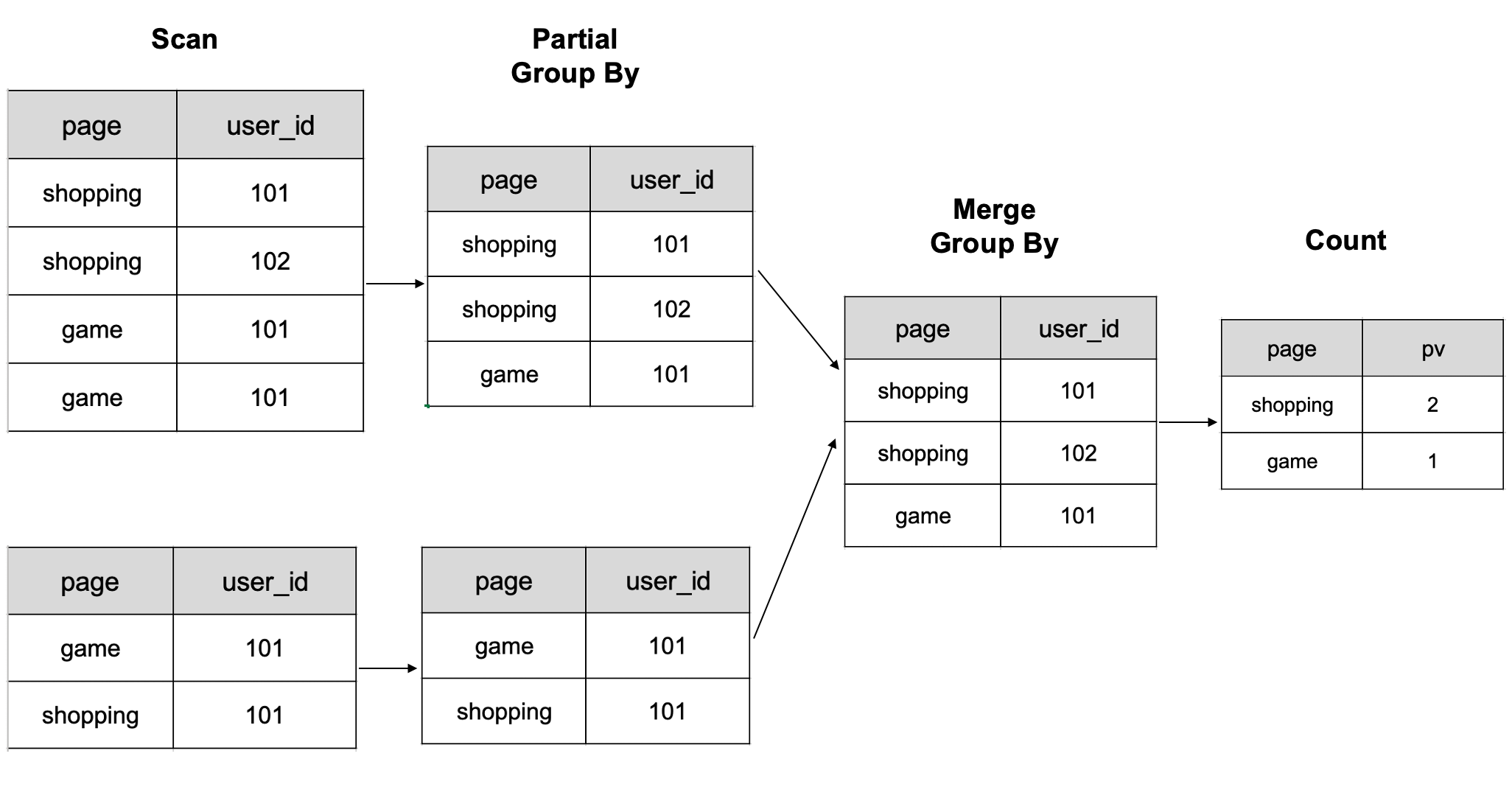
The figure shows a schematic of 6 rows of data computed on two BE nodes.

When dealing with large volumes of data that require multiple shuffle operations, the computational resources needed can increase significantly. This slows queries. However, using the Bitmap technology can help address this issue and improve query performance in such scenarios.

Count uv grouping by page:

select page, count(distinct user_id) as uv from table group by page;

page	uv
game	1
shopping	2

Benefits of Count Distinct with Bitmap

You can benefit from bitmaps in the following aspects compared with COUNT(DISTINCT expr):

• Less storage space: If you use bitmap to compute the number of distinct values for INT32 data, the required storage space is only 1/32 of COUNT(DISTINCT expr). Compressed roaring bitmaps are used to execute computations, further reducing storage space usage compared to traditional bitmaps.
• Faster computation: Bitmaps use bitwise operations, resulting in faster computation compared to COUNT(DISTINCT expr). Computation of the number of distinct values can be processed in parallel, leading to further improvements in query performance.

For the implementation of Roaring Bitmap, see specific paper and implementation.

Usage notes

• Both bitmap indexing and bitmap Count Distinct use the bitmap technique. However, the purpose for introducing them and the problem they solve are completely different. The former is used to filter enumerated columns with a low cardinality, while the latter is used to calculate the number of distinct elements in the value columns of a data row.
• You can define a value column as BITMAP regardless of the table types (Aggregate table, Duplicate Key table, Primary Key table, or Unique Key table). However, the sort key of a table cannot be of the BITMAP type.
• When creating a table, you can define the value column as BITMAP and the aggregate function as BITMAP_UNION.
• You can only use roaring bitmaps to compute the number of distinct values for data of the following types: TINYINT, SMALLINT, INT, and BIGINT. For data of other types, you need to build global dictionaries.

Count Distinct with Bitmap

Take the calculation of page UVs as an example.

1. Create an Aggregate table with a BITMAP column visit_users, which uses the aggregate function BITMAP_UNION.

   CREATE TABLE `page_uv` (
     `page_id` INT NOT NULL COMMENT 'page ID',
     `visit_date` datetime NOT NULL COMMENT 'access time',
     `visit_users` BITMAP BITMAP_UNION NOT NULL COMMENT 'user ID'
   ) ENGINE=OLAP
   AGGREGATE KEY(`page_id`, `visit_date`)
   DISTRIBUTED BY HASH(`page_id`)
   PROPERTIES (
     "replication_num" = "3",
     "storage_format" = "DEFAULT"
   );

2. Load data into this table.

   Use INSERT INTO to load data:

   INSERT INTO page_uv VALUES
   (1, '2020-06-23 01:30:30', to_bitmap(13)),
   (1, '2020-06-23 01:30:30', to_bitmap(23)),
   (1, '2020-06-23 01:30:30', to_bitmap(33)),
   (1, '2020-06-23 02:30:30', to_bitmap(13)),
   (2, '2020-06-23 01:30:30', to_bitmap(23));

   After data is loaded:

   • In the row page_id = 1, visit_date = '2020-06-23 01:30:30', the visit_users field contains three bitmap elements (13, 23, 33).
   • In the row page_id = 1, visit_date = '2020-06-23 02:30:30', the visit_users field contains one bitmap element (13).
   • In the row page_id = 2, visit_date = '2020-06-23 01:30:30', the visit_users field contains one bitmap element (23).

3. Calculate page UVs.

   SELECT page_id, count(distinct visit_users)
   FROM page_uv GROUP BY page_id;

   +-----------+------------------------------+
   |  page_id  | count(DISTINCT `visit_users`)|
   +-----------+------------------------------+
   |         1 |                            3 |
   |         2 |                            1 |
   +-----------+------------------------------+
   2 row in set (0.00 sec)

Global Dictionary

Currently, the Bitmap-based Count Distinct mechanism requires the input to be an integer. If the user needs to use other data types as input to the Bitmap, then the user needs to build their own global dictionary to map other types of data (such as string types) to integer types. There are several ideas for building a global dictionary:

Hive table-based Global Dictionary

The global dictionary itself in this scheme is a Hive table, which has two columns, one for raw values and one for encoded Int values. The steps to generate the global dictionary are as follows:

1. De-duplicate the dictionary columns of the fact table to generate a temporary table
2. Left join the temporary table and the global dictionary, add new value to the temporary table.
3. Encode the new value and insert it into the global dictionary.
4. Left join the fact table and the updated global dictionary, replace the dictionary items with IDs.

In this way, the global dictionary can be updated and the value columns in the fact table can be replaced using Spark or MR. Compared with the trie tree-based global dictionary, this approach can be distributed and the global dictionary can be reused.

However, there are a few things to note: the original fact table is read multiple times, and there are two joins that consume a lot of extra resources during the calculation of the global dictionary.

Build a global dictionary based on a trie tree

Users can also build their own global dictionaries using trie trees (also known as prefix trees or dictionary trees). The trie tree has common prefixes for the descendants of nodes, which can be used to reduce query time and minimize string comparisons, and therefore is well suited for implementing dictionary encoding. However, the implementation of trie tree is not easy to distribute and can create performance bottlenecks when the data volume is relatively large.

By building a global dictionary and converting other types of data to integer data, you can use Bitmap to perform accurate Count Distinct analysis of non-integer data columns.